Intro

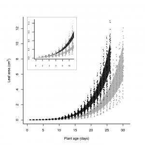
Figure 1. Arabidopsis rosettes displaying power-law growth. The grey is a mutant genotype that grows more slowly. Notice that the variance increases through time, although fitting individual plant as a random effect often removes this problem. Figure courtsey of Tobias Zust

Plant growth usually follows a non-linear trajectory, which makes linear modeling unsuitable. Fortunately, it’s really not that difficult to fit non-linear models thanks to recent libraries developed for the R statistical software. Both nlme and gnls are useful and normally work well. You will need nlme if you have repeated measures on individuals, for example, if you have recorded size in a non-destructive way on the same individuals at regular points in time. If you only have destructive harvests (so one measure per individual), then gnls might be more appropriate.

Choosing a curve

This depends on the nature of your data. Plot your data first and have a look! It’s amazing how often people don’t do this. Does your data show evidence of a clear asymptote? If yes, then a logistic or asymptotic function might be appropriate. If no, then perhaps your data follows a power law (see Figure 1). For many of the non-linear functions, self-starting routines exist which make model convergence easier, e.g. SSlogis. The power-law model does not have a self-starting routine and doesn’t always converge well, but there’s code in a recent methods paper we wrote that includes this function. You might also consider transforming your data. A log-transformation usually works well and has the added advantage of dealing with the problem of increasing variance (see Figure 1). However, we have found that if you have repeated non-destructive size measures on individuals and hence can include individual as a random effect, the residual errors no longer display this problem. This makes sense because variation in growth rate among individuals creates the problem in the first place; so fitting this effect will often remove it.

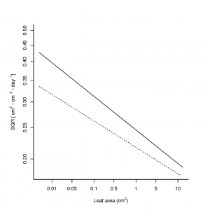
Figure 2. Size-standardised growth rates (SGR) decline with plant size. Figure courtesy of Tobias Zust.

Calculating growth rates

Once you’ve fitted your curves, it’s easy to calculate growth rates. We recommend calculating size-standardized growth rates as this facilitates comparisons among species. For example, small plants just usually grow faster than large ones. So especially if you grew your plants from seed the small-seeded plants will all appear to be very fast growing. However, if you want to know whether they can maintain this growth advantage, you need to compare them at the same size.  Once again, in our recent methods paper you can find the formulae to calculate size-standardized growth rates for a large range of potential functions.